Comparison of rhs! Performance: CPU vs. GPU

This documentation serves as a supplementary material for JuliaCon 2025.

See the benchmarking file at benchmark.ipynb, and all results are compared between TrixiCUDA.jl v0.1.0-rc.3 and Trixi.jl v0.11.17. All the benchmark examples can be found in the benchmark directory.

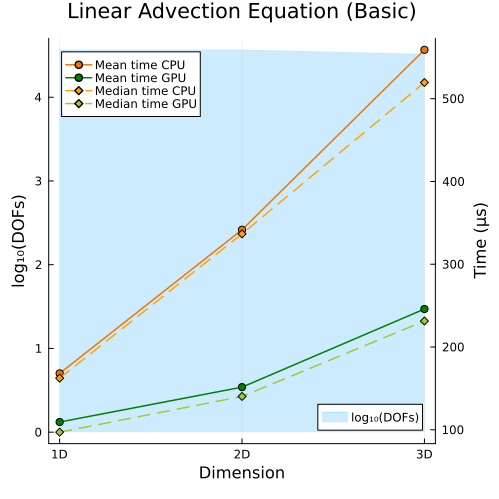
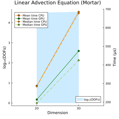
We mainly show the mean and median times on CPU and GPU for each example, and include the degrees of freedom (DOFs) per field (i.e., per independent solution variable) in each plot, since DOFs are a dominant factor (though not the only factor) affecting computational time.

We provide the link to each example in Trixi.jl as it is a more mature and stable package compared to TrixiCUDA.jl. Note that performance varies with different inputs; these benchmark results are provided for reference only.

Approaches

We adopt two approaches here:

• First, we maintain a consistent solution resolution per space dimension by fixing both the degree of polynomial basis (i.e., polydeg) and mesh refinement level (i.e., initial_refinement_level), while varying the problem dimension from 1D to 2D to 3D. In this way, we observe a linear increase in log DOFs with problem dimension.

• Second, for each problem type, we keep the number of DOFs roughly constant across 1D, 2D, and 3D by changing the polynomial degree (i.e., polydeg) and mesh refinement level (i.e., initial_refinement_level). This way produces a roughly flat log DOFs curve across all dimensions.

We will present benchmark results for two approaches.

Results

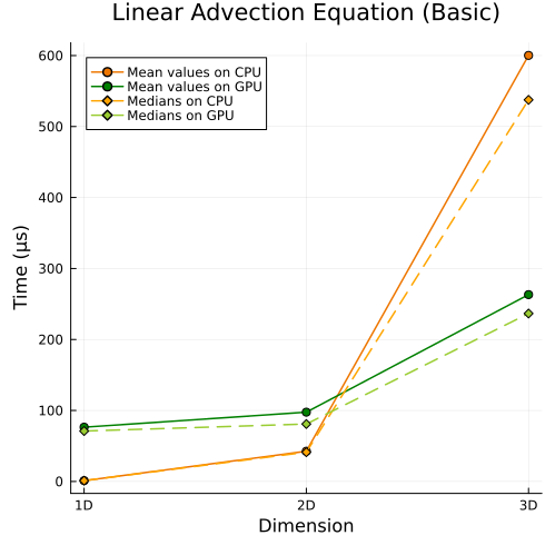
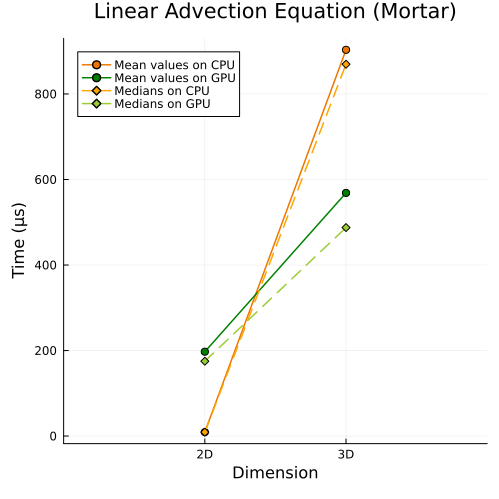
Linear Advection Equation

Left: Basic linear advection equation (1D, 2D, 3D)
Right: Linear advection equation with mortar method (2D, 3D)

• First approach

• Second approach

Compressible Euler Equations

Left: Compressible Euler equations with entropy-conservative flux (1D, 2D, 3D) Right: Compressible Euler equations with shock capturing (1D, 2D, 3D)

• Fisrt approach

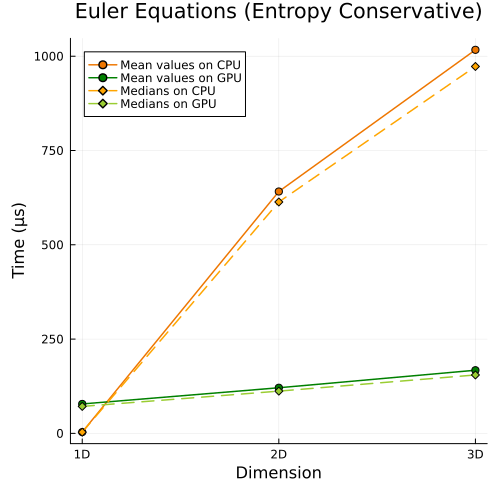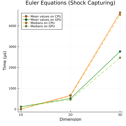• Second approach

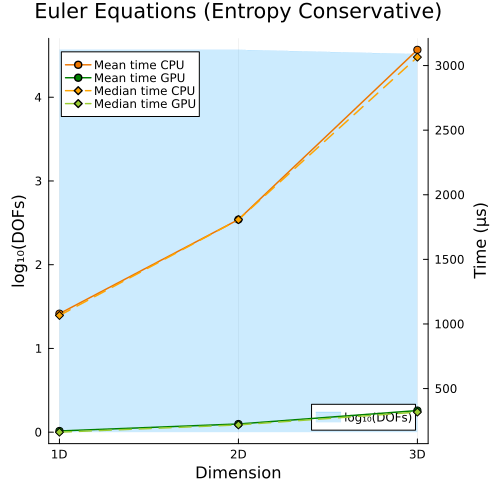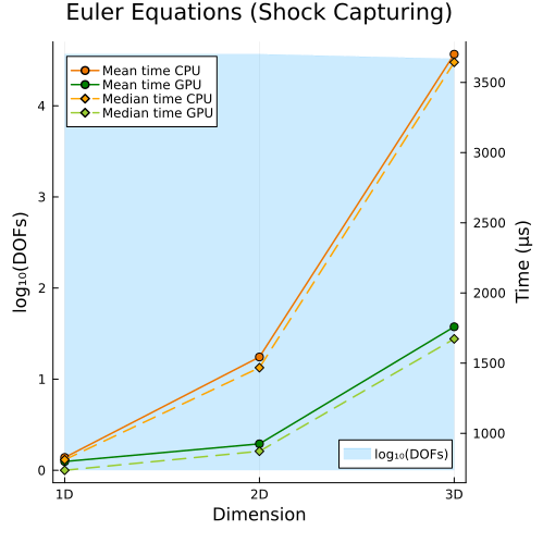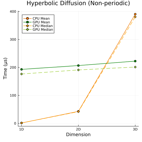
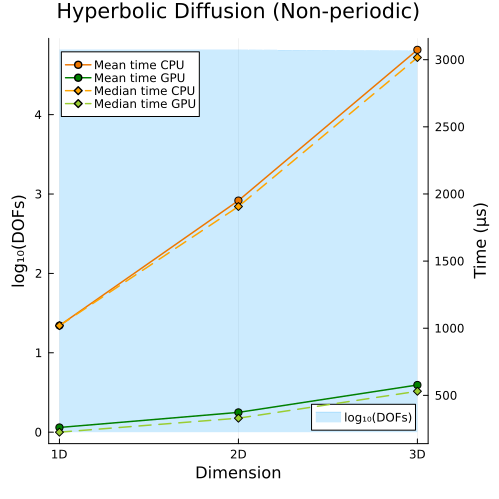
Hyperbolic Diffusion Equations

Hyperbolic diffusion equations with non-periodic boundary conditions (1D, 2D, 3D)

• First approach

• Second approach

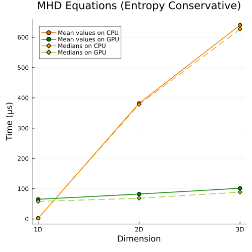
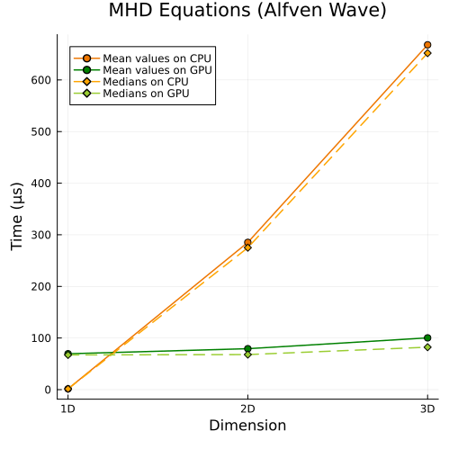
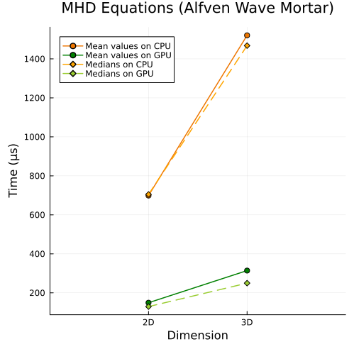
Ideal GLM-MHD Equations

Upper: Ideal GLM-MHD equations with entropy-conservative flux (1D, 2D, 3D)
Lower left: Ideal GLM-MHD Alfven wave (1D, 2D, 3D)
Lower right: Ideal GLM-MHD Alfven wave with mortar method (2D, 3D)

• First approach

• Second approach

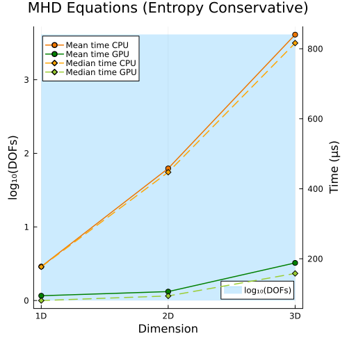
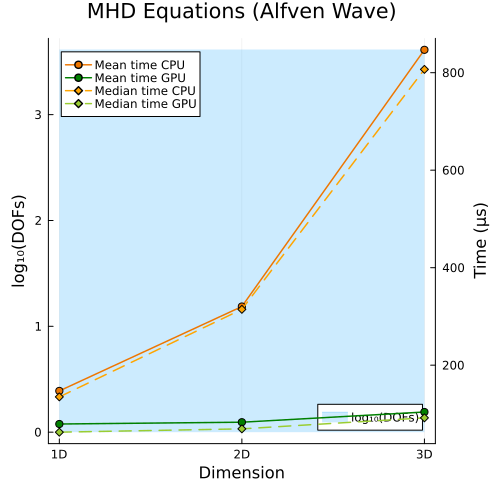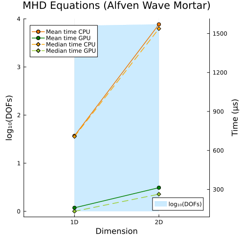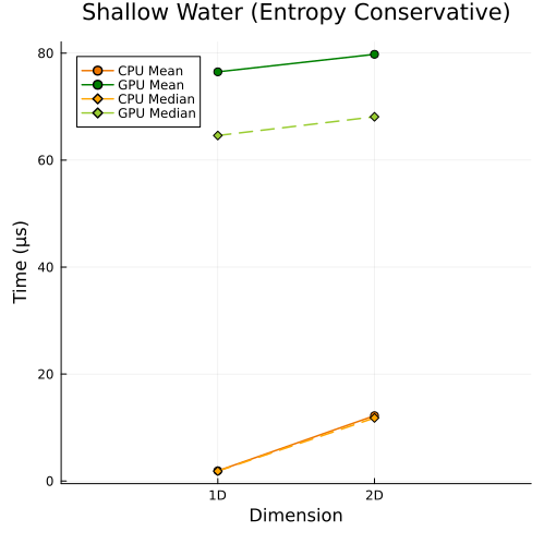
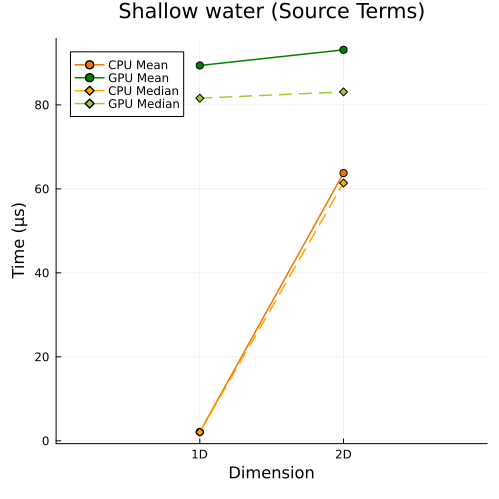
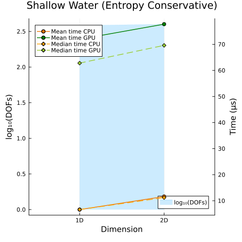
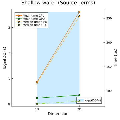
Shallow Water Equations

Left: Shallow water equations with entropy conservative flux (1D, 2D)
Right: Shallow water equations with source terms (1D, 2D)

• First approach

• Second approach

Takeaway

In the first approach, CPU and GPU runtimes both rise as DOFs increase, simply because more unknowns must be solved; while in the second approach, even when the total DOFs are held roughly constant, CPU and GPU runtimes still increase with problem size, since the cost of solving each unknown also grows with the spatial dimension of the problem.

However, in both approaches, we observe that the slope of the runtime on the GPU is smaller than that on the CPU, so the GPU is less sensitive to increases in data size and thus robust in handling large-scale problems. So, we can conclude that the speedup increases with the problem size (including both the number of spatial dimensions and the level of solution resolution).